Back to Gallery | Home

GIF Animations / GIFアニメーション

0: $N$th roots of complexes / 複素数の $N$乗根
1: Euler's formula / オイラーの公式
2: Differentials and linear approximation / 微分と1次近似
3: Riemann integral / リーマン積分
4: Lebesgue integral / ルベーグ積分
5: Definition of area / 面積の定義
6: Surface area / 曲面積
7: Fourier series / フーリエ級数
8: Frenet-Serret frames / フルネ・セレ標構
9: $L^p$ convergence / $L^p$ 収束
10: Complex line integral / 複素線積分

0. $N$th roots of complexes / 複素数の $N$乗根

For a given complex number $A=r e^{i \theta} =r (\cos \theta + i \sin \theta) \neq 0$, its $N$th roots (i.e., solution of the equation $z^n=A$) are given by $$ \sqrt[N]{r} e^{i \theta/N} \omega^k $$ where $\omega=e^{2 \pi i/N}$ and $k=0,1,\ldots, N-1$. This GIF animation depicts the $N$th roots (blue dots) of the red dot $A$ making one turn around the origin for $N=2,3,4,5,6$.
複素数 $A=r e^{i \theta} =r (\cos \theta + i \sin \theta) \neq 0$ に対し，その $N$乗根（方程式 $z^n=A$ の解）は $$ \sqrt[N]{r} e^{i \theta/N} \omega^k $$ （ただし，$\omega=e^{2 \pi i/N}$ かつ $k=0,1,\ldots, N-1$） で与えられる．. この GIF アニメーションは，原点のまわりを1周する点 $A$ の$N$乗根を$N=2,3,4,5,6$ に対し図示したものである．

1. Euler's formula / オイラーの公式

LEFT: The complex exponential function $e^z=\exp z$ is defined by the series $\displaystyle e^z = 1 + \frac{z}{1!}+\frac{z^2}{2!}+\cdots $ for each $z \in \mathbb{C}$. When we let $z = it$ with $t \in \mathbb{R}$, the celebrated Euler's formula $e^{it}=\cos t + i \sin t$ follows. Indeed, the sequence $\{z_n\}$ defined by the recursive formula $\displaystyle z_0=0; z_{n+1}=z_{n} + \frac{(it)^n}{n!} $ converges to $\cos t + i \sin t$, a point on the unit circle. This GIF animation depicts the convergence of the sequence $\{z_n\}$ (blue heavy dots joined by blue segments) with angular parameter $t$ increasing from 0 to $4 \pi$.
RIGHT: The same idea applied for $z=\log 2 + i t~(0 \le t \le 4 \pi)$.
左: 複素数 $z \in \mathbb{C}$ に対し， 複素指数関数 $e^z=\exp z$ は 級数 $\displaystyle e^z := 1 + \frac{z}{1!}+\frac{z^2}{2!}+\cdots $ によって定義される．とくに，$z = it$（$t \in \mathbb{R}$）を代入したとき， 有名な オイラーの公式 $e^{it}=\cos t + i \sin t$ が得られる. 実際，数列 $\{z_n\}$ を漸化式 $\displaystyle z_0=0; z_{n+1}=z_{n} + \frac{(it)^n}{n!} $ によって定義するとき，これは単位円周上の点 $\cos t + i \sin t$ に収束する． この GIF アニメーションは， 角度のパラメーター $t$ を 0 から $4 \pi$ まで動かしたとき， 数列 $\{z_n\}$ （青い線で結ばれる青い点たち） が収束する様子を表現したものである．
右:同様に $z=\log 2 + i t~(0 \le t \le 4 \pi)$ としたもの.

2. Differentiation and linear approximation / 微分と1次近似

LEFT: We say a function $y=f(x)$ is differentiable at $x=a$ if there exists a constant $A \in \mathbb{R}$ such that $\displaystyle f(x)= f(a)+A (x-a) + o(x-a)~~(x \to a). $ This means that $f(x)$ is approximated by the tangent line $y = f(a) + A (x-a)$ and its relative precision gets better as $x \to a$. In other words, if we magnify the graph of $y=f(x)$ at $(a, f(a))$, it becomes harder to distinguish it from the tangent line. In this GIF animation $f(x)=\sin 3x + \sin^2 5x$, $a=0$, and $A=3$.
RIGHT: We say a function $z=f(x, y)$ in two variable is differentiable at $(x,y)=(a,b)$ if there exists a vector $(A, B) \in \mathbb{R}^2$ such that $\displaystyle ~~~~~~~~f(x,y)= f(a,b)+A (x-a) + B(y-b)+o(\{(x-a)^2+(y-b)^2\}^{1/2}) $
as $(x,y) \to (a,b).$ Instead of considering the tangent plane, we use contour graphs to understand what it means. The contours (level curves) of $z=f(a,b)+A (x-a) + B(y-b)$ are straight lines perpendicular to the gradient vector $(A,B)$. Hence the differentiability means the contours of $z=f(x,y)$ are approximated by those of $z=f(a,b)+A (x-a) + B(y-b)$. In this GIF animation $f(x,y)=\sin(x + y)\cos( y - x^2/3 + 2)$, $(a,b)=(0,0)$, and $(A,B)= (\cos 2,\cos 2)$.
左: 関数 $y=f(x)$ が $x=a$ で 微分可能 であるとは， ある定数$A \in \mathbb{R}$ が存在し， $\displaystyle f(x)= f(a)+A (x-a) + o(x-a)~~(x \to a). $ が成り立つことをいう．すなわち， $f(x)$ は接線 $y = f(a) + A (x-a)$ によって近似され，その相対的な精度は $x \to a$ のときより高くなる． 言い換えると，$y=f(x)$ のグラフを点 $(a, f(a))$ を中心に 拡大すればするほど，接線との区別が難しくなるということである． この GIF アニメーションでは， $f(x)=\sin 3x + \sin^2 5x$, $a=0$, $A=3$ としている．
右: 2変数関数 $z=f(x, y)$ が $(x,y)=(a,b)$ において 微分可能 であるとは，あるベクトル $(A, B) \in \mathbb{R}^2$ が存在し，$(x,y) \to (a,b)$ のとき $\displaystyle ~~~~~~~~f(x,y)= f(a,b)+A (x-a) + B(y-b)+o(\{(x-a)^2+(y-b)^2\}^{1/2}) $
となることをいう． その意味するところを理解するには，接平面を考えるよりも， 等高線グラフを考えるほうがよい． 関数 $z=f(a,b)+A (x-a) + B(y-b)$ の等高線はその勾配ベクトル $(A,B)$ と垂直な直線たちになる． よって，$z=f(x,y)$ の微分可能性とは， その等高線が $z=f(a,b)+A (x-a) + B(y-b)$ の等高線によって近似される， ということである． この GIF アニメーションでは， $f(x,y)=\sin(x + y)\cos( y - x^2/3 + 2)$, $(a,b)=(0,0)$, and $(A,B)= (\cos 2,\cos 2)$ としている.

3. Riemann Integral / リーマン積分

LEFT: In the 19th century Riemann introduced a classical definition of integration which is still fundamental in college mathematics and numerical analysis. The idea is to approximate the region between the graph of a function and the axis by thin rectangles. In this animation the approximation starts with 5 rectangles (with randomly chosen thickness) and it gets finer as the number of rectangles increases up to 100.
MIDDLE and RIGHT: The same idea is applied for multivariable functions. For functions with two variables we use thin cuboids (like square columns) for approximation.
左: 19世紀にリーマンが与えた積分の古典的な定義は， 現在も大学教養課程における数学や，数値解析学における基礎となっている． そのアイディアは，関数のグラフと軸で囲まれる部分を細長い長方形によって近似する， というものである．このアニメーションでは，5つの長方形（太さはランダムに選んでいる） による近似からスタートし，長方形の数が100まで増加する過程で近似が改善される様子を表している．
中央と右: 多変数の関数に対しても同様のアイディアが適用できる． 2変数の場合は，近似に細い直方体（角柱）を用いるのである．

4. Lebesgue Integral / ルベーグ積分

LEFT: Analysis in the 20th century started with a novel definition of integration by Lebesgue that extends Riemann's. The Lebesgue integral is very importnat but it is a bit tricky to depict the idea. (Indeed, there are some misleading pictures that seem, in my opinion, drawn incorrectly.) For example, let us take a continuous function $f:[a,b] \to [m, M]$ and let $\mu(A)$ denote the one dimensional Lebesgue measure ("length") of the set $A \subset \mathbb{R}$. Lebesgue's excellent idea is to regard the sum $$ \sum_{k=0}^{N-1} y_k \cdot \mu(\{x \in [a,b] \mid y_k \le f(x) < y_{k+1} \}) $$ with a very fine division $m = y_0 < y_1 < \cdots < y_N = M$ of the range $[m,M]$ as an approximation of the desired integration. The set $\{x \in [a,b] \mid y_k \le f(x) < y_{k+1} \}$ usually consists of fragments of intervals and the value $y_k \cdot \mu(\{x \in [a,b] \mid y_k \le f(x) < y_{k+1} \})$ is the total "area" of the columns (thin rectangles) of height $y_k$ over these fragments. The advantage of this formulation is that we can apply it to a fairly large class of functions that might have discontinuity or very strong oscillation. Practically we evenly divide the range and by increasing the number $N$ of division the columns gradually fill the region enclosed by the axis and the graph of the function $f$. In this animation, we take $f(x)=(\sin x + \cos^2 4x)/2$ with $0 \le x \le \pi/2$ and $N$ ranges over $2$ to $50$. The colors of columns distinguish their heights.
In the animation below, the same idea is applied to a function in two variables.
RIGHT: It is more practical to take a increasing sequence of "step functions" to approximate the graph of the original function $f$. Here we choose $N=2, 4, 8, \cdots, 64$ to obtain an increasing sequence in the same setting as LEFT.
左: 20世紀の解析学は，ルベーグによる新しい積分論とともに始まった． リーマン積分を拡張したルベーグの積分は非常に重要な概念だが， 図解しようと思うと，意外と厄介であることに気づく （実際，間違ってるのでは？という感じの 図 もよく見かける）． 例えば，連続関数 $f:[a,b] \to [m, M]$ をひとつとり， 記号 $\mu(A)$ で集合 $A \subset \mathbb{R}$ の 1次元ルベーグ測度（「長さ」）を表すものとする． ルベーグの秀逸なアイディアは， まず値域 $[m,M]$ を十分に細かく分割する値 $m = y_0 < y_1 < \cdots < y_N = M$ を決めて， それから定まる和 $$ \sum_{k=0}^{N-1} y_k \cdot \mu(\{x \in [a,b] \mid y_k \le f(x) < y_{k+1} \}) $$ を定義したい積分を近似する量とみなしたことにある． 集合 $\{x \in [a,b] \mid y_k \le f(x) < y_{k+1} \}$ は通常， 細切れの区間の集まりとなるから， 値 $y_k \cdot \mu(\{x \in [a,b] \mid y_k \le f(x) < y_{k+1} \})$ は細切れの区間たちの上に立つ高さ $y_k$ の柱（細長い長方形）たちの 面積和だと考えられる． 同様のアイディアは不連続関数や振動の激しい関数を含む極めて広いクラスの関数に対しても適用でき，それがルベーグによる定式化の強みとなっている． 実用上は値域の分割幅を一定にし，その分割数 $N$ を増やすことで柱たちが関数 $f$ のグラフと横軸で囲まれる領域を次第に満たしていくようにとる． このアニメーションでは，$0 \le x \le \pi/2$ 上の 関数 $f(x)=(\sin x + \cos^2 4x)/2$ を考え， $N$ は $2$ から $50$ まで変化させている. 柱の色の違いは，柱の高さの違いを表現している．
この下のアニメーションは，同じアイディアを2変数関数に適用したものである．
右: より実用的な定義として，関数 $f$（の値が正の部分）を「単調増加な階段関数の列」によって近似する，という方法がある．ここでは，左のアニメにおける分割数を $N=2, 4, 8, \cdots, 64$ と順に増やすことで，単調増加になるようにしている．

5. Definition of area / 面積の定義

Areas of plane sets are defined by means of 2 dimensional Lebesgue measure in modern mathematics, but it is still common to teach the classical and naive notion of area à la Jordan in college mathematics. It is a good bi-product of the definition of Riemann integral, and hence it goes well with numerical analysis.
For a given bounded set $A \subset \mathbb{R^2}$, we define its characteristic function $\chi_A:\mathbb{R}^2 \to \{0, 1\}$ by $$ \chi_A(x,y) := \left\{\begin{array}{ll} 1 & ((x,y) \in A)\\ 0& ((x,y) \in \mathbb{R}^2 -A)\end{array} \right.. $$ Now suppose that the function $\chi_A$ is Riemann integrable, i.e., the Riemann integral $$ m(A) = \int_{\mathbb{R}^2} \chi_A(x,y) \,dx dy $$ has a definite non-zero value. It is known that it is equivalent to the condition that $A$ is Jordan measurable, and the value $m(A)$ coincides with the classical Jordan measure of $A$. Hence we can define the Jordan measure ("area à la Jordan") of $A$ by the integral $m(A)$ (if it exists). In general, a bounded set $A$ is Jordan measurable if and only if its boundary $\partial A$ is a null set in the sense of Lebesgue, and $m(A)$ coincides with 2 dimensional Lebesgue measure of $A$. In this gif animation, we approximate the characteristic function of a set $A$ bounded by a complicated fractal set (orange dots) according to the definition of Riemann integral. Even if a block intersect with the set $A$, there is no yellow cuboid of height one over the block if the representation point of the Riemann sum is chosen outside $A$. By refining the blocks, such an unlucky blocks are pushed away to the boundary and we will obtain an accurate approximation of the area.
平面集合の面積は2次元ルベーグ測度によって定式化するのが現代的だが， 大学初年級の数学では古典的かつ素朴なジョルダン流の面積概念もよく教えられている． リーマン積分を定義する際に副産物として得られる点は嬉しいし， それゆえに数値計算との相性もよい． 与えられた有界集合 $A \subset \mathrm{R^2}$ に対し， 特性関数 $\chi_A:\mathbb{R}^2 \to \{0, 1\}$ を $$ \chi_A(x,y) := \left\{\begin{array}{ll} 1 & ((x,y) \in A)\\ 0& ((x,y) \in \mathbb{R}^2 -A)\end{array} \right. $$ と定義する． このとき，関数 $\chi_A$ がリーマン可積分であること， すなわち，リーマン積分 $$ m(A) = \int_{\mathbb{R}^2} \chi_A(x,y) \,dx dy $$ が有限の値で定まることは， 集合 $A$ がジョルダン可測であることと同値であり， しかも $m(A)$ が $A$ のジョルダン測度と一致することが知られている． したがって，この積分値を（それがもし存在すれば）集合 $A$ のジョルダン測度（「ジョルダン流の面積」）として定義してもよいのである． 一般に，境界 $\partial A$ がルベーグの意味で零集合であれば （例えば，私たちが初等幾何学で扱うような図形であれば） ジョルダン可測であり， 「面積」の値も2次元ルベーグ測度と一致する． この gif アニメーションは，複雑なフラクタル集合（オレンジの点たち）で 囲まれた集合 $A$ の特性関数をリーマン積分の定義に基づいて近似する 様子を視覚化したものである．集合 $A$ と交わる区画であっても， リーマン和の代表点が $A$ に入らなければ「黄色い角柱」は立てられない． 区画を細分することで，そうした不運な区画は 境界部分に押しやられていき，結果的に正しい面積が近似計算できるのである．

6. Surface area / 曲面積

Defining the ``area" of a given surface is quite non-trivial. If the surface is smooth, then we have a natural definition by integration. For example, let $S$ be a surface parametrized by a vector-valued smooth (or $C^1$) function $\vec{p}=\vec{p}(s,t) \in \mathbb{R}^n$ where $(s,t)$ ranges over a domain $D$ of $\mathbb{R}^2$. Then its area is defined by $\displaystyle \iint_D \left ||\vec{p}_s\times\vec{p}_t \right || \, ds \, dt$. The integration is a limit of the total areas of tiny tangent planes (panels).
曲面に対し「面積」を定義するのはそれほど簡単ではない． しかし，曲面が滑らかであれば，積分を用いた自然な定義が知られている． たとえば，曲面 $S$ が滑らかな（あるいは $C^1$級の）ベクトル値関数 $\vec{p}=\vec{p}(s,t) \in \mathbb{R}^n$ （ただし $(s,t)$ は $\mathbb{R}^2$ 内の領域 $D$ 内を動くものとする） でパラメーター表示されるとき，その面積は $\displaystyle \iint_D \left ||\vec{p}_s\times\vec{p}_t \right || \, ds \, dt$. によって定義される．この積分は，微小な接平面たちの，総面積の極限になっている．

7. Fourier Series / フーリエ級数

Let $f:\mathbb{R} \to \mathbb{R}$ be a square wave function, that is, a periodic function of period $2 \pi$ such that
$f(x)=-1~(-\pi < x \le 0)$ and $f(x)=1~(0< x \le \pi)$. By a classical result on Fourier series due to Dirichlet, it follows that that the equation \[ f(x)=\frac{4}{\pi}\Big( \sin x + \frac{\sin 3x}{3}+ \frac{\sin 5x}{5}+\cdots\Big) =\lim_{N \to \infty} \sum_{n=-N}^N \frac{-2i}{(2n-1)\pi}\big\{e^{(2n-1) xi} - e^{-(2n-1) xi}\big\} \] holds unless $f$ is discontinuous at $x$. The middle one is the Fourier expansion and the right-most one is its complex form. This animation shows the motion of the finite sum \[ S_N(x):=\frac{-2i}{\pi} \Big\{e^{xi} -e^{-xi} + \frac{e^{3xi}}{3} - \frac{e^{-3xi}}{3} +\cdots +\frac{e^{(2N-1)xi}}{2N-1} - \frac{e^{-(2N-1)xi}}{2N-1} \Big\} \] for sufficiently large $N$. Since $e^{\pm (2N-1)xi}$ rotates along the unit circle $\pm(2N-1)$ times for each period $2 \pi$, $S_N(x)$ is a composition of rotations with distinct weights. The animations below shows the case for $N=1,3$ and $5$.
周期 $2\pi$ をもつ矩形波関数 $f:\mathbb{R} \to \mathbb{R}$ を $f(x)=-1~(-\pi < x \le 0)$，$f(x)=1~(0< x \le \pi)$ が成り立つように定義する（すなわち，$(-\pi,\pi]$ 以外では 周期性 $f(x+2 \pi)=f(x)$ を用いて拡張する）． フーリエ級数に関する古典ともいえる ディリクレの定理によれば，不連続点を除いて等式 \[ f(x)=\frac{4}{\pi}\Big( \sin x + \frac{\sin 3x}{3}+ \frac{\sin 5x}{5}+\cdots\Big) =\lim_{N \to \infty} \sum_{n=-N}^N \frac{-2i}{(2n-1)\pi}\big\{e^{(2n-1) xi} - e^{-(2n-1) xi}\big\} \] が成立する．中央の級数がいわゆる フーリエ展開 であり，最後の級数はその複素形を与える． このアニメーションは，$x$ を時間のパラメーターとして， 有限和 \[ S_N(x):=\frac{-2i}{\pi} \Big\{e^{xi} -e^{-xi} + \frac{e^{3xi}}{3} - \frac{e^{-3xi}}{3} +\cdots +\frac{e^{(2N-1)xi}}{2N-1} - \frac{e^{-(2N-1)xi}}{2N-1} \Big\} \] の動きを十分に大きな $N$ に対して描画したものである． $e^{\pm (2N-1)xi}$ は時間 $2\pi$ で単位円上を $\pm(2N-1)$周する動きを表すから， これは速度の異なる円運動を重みつきで合成したものとなる． 下の図は $N=1, 3, 5$ について $S_N(x)$ の動きを表現したものである．

8. The Frenet-Serret frames / フルネ・セレ標構

9. $L^p$ convergence / $L^p$ 収束

It is hard to imagine the topology of the $L^p$ space $L^p([0,1])$ for $p \ge 1$, that is, the vector space of functions $f(x)$ on $[0,1]$ whose Lebesgue norm $\displaystyle ||f(x)||=\Big (\int_0^1 |f(x)|^p \, dx \Big)^{1/p}$ is finite. The animation depicts a sequence of functions $\{f_n\}$ such that it converges to $f \equiv 0$ (the zero vector) in $L^p$ but the sequence of numbers $\{f_n(x)\}$ diverges for every $x \in [0,1]$.
$L^p$ 空間 $L^p([0,1])$（$p \ge 1$）とは， $[0,1]$区間上の関数 $f(x)$ で，ルベーグのノルム $\displaystyle ||f(x)||=\Big (\int_0^1 |f(x)|^p \, dx \Big)^{1/p}$ が有限となるもの全体からなるベクトル空間だが， その位相を思い描くのはなかなか難しい． このアニメーションでは，関数列 $\{f_n\}$ で，$L^p$ において $f \equiv 0$ （0ベクトル）に収束するが， 任意の点 $x \in [0,1]$ で数列 $\{f_n(x)\}$ が発散するようなものを表現している．

10. Complex line integral / 複素線積分

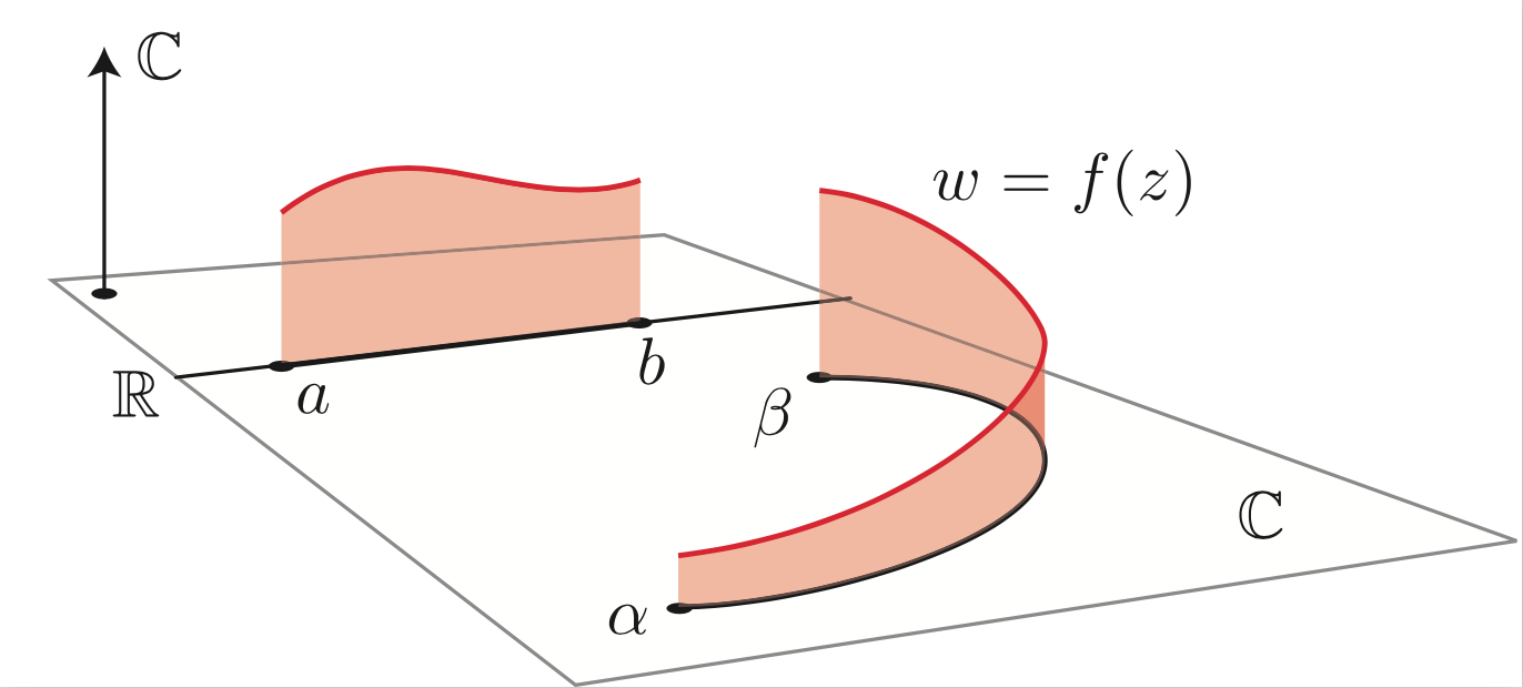
The animations above are drawn numerically by following the rigorous, mathematical definitions. However, the animation here (LEFT) is an exception.
When I teach complex analysis, I draw a picture like the one on the right and say "complex line integral is a natural extension of definite (Riemann) integrals of real functions". I made this animation to show the idea even more expressively.
We put thin rectangles over the segments approximating the path to make a "folding screen". The height of each rectangle is a complex number that is the value of the complex function to integrate. We may regard the complex line integral as the limit of the "complex area" of this "folding screen".
これまでのアニメーションはすべて数学的に厳密な定義に基づき， できるだけ忠実に数値計算させて描いたものだが， ここでお見せするもの（左側）だけはちょっと事情が違う．
私は複素関数論の講義で，「複素線積分は実関数の定積分（リーマン積分） の自然な拡張です」といって，右側のようなイメージ図を描くことにしていて （そして＜イメージです＞と書き添える）， その気分をより豊かに伝えるために作ったのが左側のgifアニメーションである．
曲線を近似する折れ線の上に短冊（細長い長方形）を立てて， 「屏風」が作られていく． 各短冊の高さは積分される複素関数の値（もちろん複素数）である． こうして得られる「屏風」の「複素面積」が複素線積分である，と考えるのである．

Back to Gallery | Home