 fig 1
fig 1
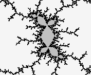 fig 2
fig 2
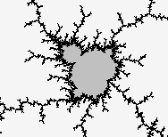 fig 3
fig 3
OTIS is a Java applet which shows the actions of quadratic functions of the form f(z)=zz+C, on the complex plane. in particular, this applet can trace forward and backward orbits of any curves.
The applet starts with drawing a picture of the Julia set of f(z)=zz+C with c = i. the initial picture is bounded by a square with width 4, centered at the origin z=0. to change the parameter value c, input re c and im c in the text-boxes, or click the mandelbrot window as explained below. Press Draw Julia to draw the Julia set. To magnify the picture, first press the button Magnification Square. Next press the mouse button to choose the center of the square which will bound the region you want to magnify, and then drag the mouse and set the square bounding the region you want to magnify(fig 1). Then press Draw Julia. For more precise picture, increase the number of iteration of the calculation with the Choice-Box labeled like iteration=****. To reset the picture to the initial range (i.e. both Re z and Im z within [-2,2]), just press Reset Window.
To draw the Julia set in Binary Switch Method, check Binary Julia. (fig 1). To draw the Julia set in Distance Estimation Method, check DistEstMthd (fig 2). Check Draw Edges to emphasize the edges of the picture. (See fig 7.)
When Attracting Basin is checked, the attracting basin (if it exists) is darkly colored according to the potential levels. (See fig 1. In fig 2, it is unchecked.) It makes the program faster in general.
fig 1
fig 2
fig 3
There is a image of the Mandelbrot set on the right of the Julia set. This is for picking up the parameter value C of zz+C. By clicking the image on this Mandelbrot window, the value Re C and Im C corresponding to the mouse cursor is set to the Text-Boxes, and then the Julia set of zz+C is automatically drawn.
To change the range of the Mandelbrot window, press Magnification Square first and then choose a square in the Mandelbrot window. Press Draw Mandel to draw the picture, and press Reset Mandel to reset the range to the original.
To draw the Mandelbrot set in Distance Estimation Method, check DistEstMthd (fig 3).
The z-coordinate pointed by the mouse cursor is shown below the Text-Boxes. To see the forward orbit of this point, press the mouse button. The orbit points are drawn as orange heavy dots and joined by orange segments (fig 4). To show the orbits without joining by segments, remove the check in Segment. When Circle is checked, circles centered at the orbit points are drawn while mouse dragging. These circles approximate the image of the blue circle at the mouse cursor.
This is the significant function of OTIS. You can see the forward and backward images of any curves which you draw by the mouse.
First, press Set Marks, then drag the mouse and draw any curve you like on the Julia picture. To see the forward image of this curve by the action of f(z)=zz+C, press Forward Image. To see the next forward image, press Forward Image again. In general, the image by N-th iteration of f(z) will be shown by pressing this button N times (fig 5).
To see the backward image of the curve by the action of f(z)=zz+C, press Backward Images. That is, for each point p on the curve, two solutions of the equation zz+C=p are drawn. to see the next backward image, press Backward Images again. In general, the backward images by N-th iteration of f(z) will be shown by pressing this button N times (fig 6).
 fig 4
fig 4
 fig 5
fig 5
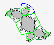 fig 6
fig 6
The option Segment also works here. Actually the marks are points joined by segments, and the number of marked points is shown below the buttons. Segment=off deactivates joining marks, and makes them thicker.
By checking ImColSwitch, the colors of forward and backward images change alternately as the number of iteration changes. (fig 6)
To clear the marks, just press Clear.
The dynamics of zz+C is approximated by that of zz near infinity. Actually they are the same in the sense of conformal dynamics. The external ray of angle p/q for zz+C corresponds to the radial ray of angle p/q for the dynamics of zz near infinity. (Angles are measured with (unit length) = (one turn). indeed, one can replace p/q by any real number.) thus the external ray of angle t is mapped to that of angle 2t. in particular, when the angle is rational, the ray naturally extends and lands on the julia set. This property helps to understand the topology of the Julia sets, and to detect the dynamics.
External rays for the Mandelbrot set are defined as follows: Parameter C outside the Mandelbrot set is on the external ray of angle t iff C is on the external ray of angle t with respect to the dynamics of zz+C. It is also known that rays of rational angles land on the Mandelbrot set.
This property is also useful for topological description of this set.
(See this note for the detail of the algorithm.)
By pressing Ext. Ray button with rational p/q (or just real t like 1.41421356..) in the text box on the right, the external rays of angle p/q (or t) for Julia and Mandelbrot sets are approximately drawn in brown (fig 7 and 8). To erase the rays, press Draw Julia or Draw Mandel. Clear does not work for this (on purpose).
The text box also accepts parameters of the form "p/q ; d" with angle p/q and positive integer d, which I call the depth of the external ray. For example, if we take d as 5, then the external ray does not land at the Julia set. If we increase d, then the end of the ray gets closer to the Julia set. Usually the default parameter d= 50 is enough deep so that the rays reach to the one-pixel neighborhood of the julia set.
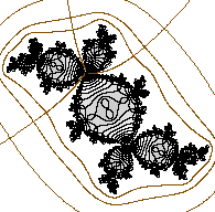 fig 7
fig 7
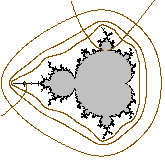 fig 8
fig 8
As a family of radial rays is perpendicular to a family of concentric circles, the family of external rays is perpendicular to a family of closed curves, called equipotential curves. Here "Equipotential" comes from a potential function on the complement of the Julia set. For example, in the dynamics of f(z)=zz, the equipotential curve of potential r is the circle of radius exp(r). note that the equipotential curve of potential r is mapped to the equipotential curve of potential 2r.
To draw the equipotential curve of potential r , use Equi. Pot button. The text box on the right accepts parameters like positive real "r" or positive rational "p/q". It also accepts "r ; s" with potential r and positive integer s, which I call sharpness. Sometimes the equipotential curve looks coarse and broken, or possibly invisible. Then there are two possibilities: (a) The potential r is too small (like r=0.00001) or too large (like r=5); or (b) too low sharpness. for (a), try r with 0.001< r < 0.5 instead. for (b), try the twice value of s instead.
When r >= 0.03, the equipotential curve of potential r of the mandelbrot set is also drawn with that of the julia set.
The orbit of z=0 ( 0, c, cc+c, (cc+c)(cc+c)+c, ...) plays very important role in the dynamics. (note that the differential is vanished only at z=0.) this orbit is called critical orbit, and shown by pressing Critical Orbit.(fig 5, points in red.)
The fixed points (points satisfying f(z)=z) also play important roles. there are two fixed points counting with multiplicity, and are shown as small yellow circles by pressing Fixed Points.
To clear these points press Clear.
-- The maximum of the number of marks is 16000.
-- See Java Applet Instructions for more general instruction.
The original version of this program, OTIS was built in 1998, my first year as a graduate student. It helped me a lot when I was learning complex dynamics. Its Java translation, OTIS-J was first built on 2001/04/15 for presentation. Then it is growing like Tubes, and in this current version, OTIS-J is renamed into OTIS again.
2004/06/19: Added DEM check-box (for "underground" seminar in Nagoya U).
2004/09/11: Added External Ray Button (for the Julia sets).
2004/12/20: External rays for the Mandelbrot set.
2005/10/09: Typing Return (Enter) Key in the text boxes works to draw Julia sets or external rays. Now Re C accepts complex values of the form a+bI with real a and b. In this case the value in Im C is ignored.
2007/10/02: Equipotential curves for the Julia sets. Added Draw Edges button.
2007/11/29: Equipotential curves for the Mandelbrot set (only for r >= 0.03).